Review: SSD — Single Shot Detector (Object Detection)
This time, SSD (Single Shot Detector) is reviewed. By using SSD, we only need to take one single shot to detect multiple objects within the image, while regional proposal network (RPN) based approaches such as R-CNN series that need two shots, one for generating region proposals, one for detecting the object of each proposal. Thus, SSD is much faster compared with two-shot RPN-based approaches.
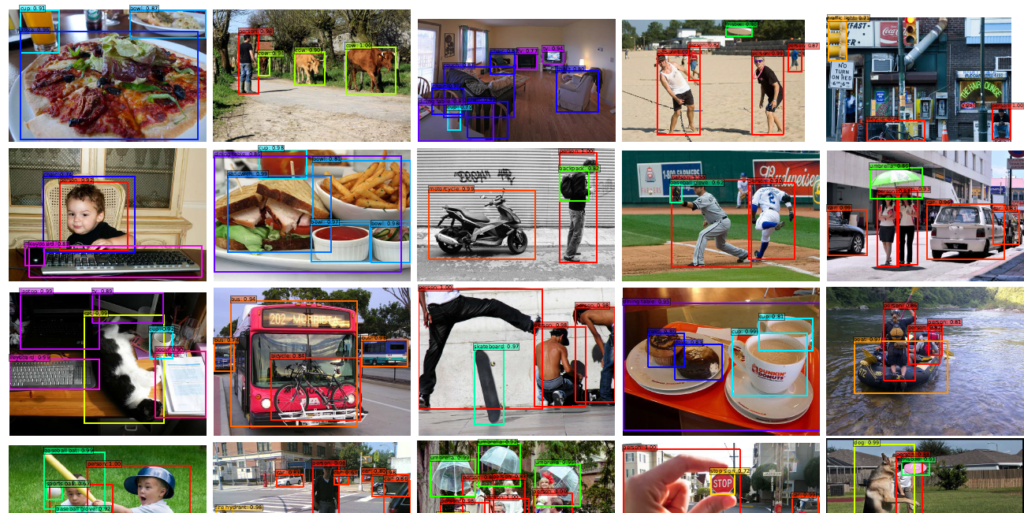
SSD300 achieves 74.3% mAP at 59 FPS while SSD500 achieves 76.9% mAP at 22 FPS, which outperforms Faster R-CNN (73.2% mAP at 7 FPS) and YOLOv1 (63.4% mAP at 45 FPS). Below is a SSD example using MobileNet for feature extraction:
From above, we can see the amazing real-time performance. And SSD is a 2016 ECCV paper with more than 2000 citations when I was writing this story. (Sik-Ho Tsang @ Medium)
What Are Covered
- MultiBox Detector
- SSD Network Architecture
- Loss Function
- Scales and Aspect Ratios of Default Boxes
- Some Details of Training
- Results
1. MultiBox Detector

- After going through a certain of convolutions for feature extraction, we obtain a feature layer of size m×n (number of locations) with p channels, such as 8×8 or 4×4 above. And a 3×3 conv is applied on this m×n×p feature layer.
- For each location, we got k bounding boxes. These k bounding boxes have different sizes and aspect ratios. The concept is, maybe a vertical rectangle is more fit for human, and a horizontal rectangle is more fit for car.
- For each of the bounding box, we will compute c class scores and 4 offsets relative to the original default bounding box shape.
- Thus, we got (c+4)kmn outputs.
That’s why the paper is called “SSD: Single Shot MultiBox Detector”. But the above it’s just a part of SSD.
2. SSD Network Architecture

To have more accurate detection, different layers of feature maps are also going through a small 3×3 convolution for object detection as shown above.
- Say for example, at Conv4_3, it is of size 38×38×512. 3×3 conv is applied. And there are 4 bounding boxes and each bounding box will have (classes + 4) outputs. Thus, at Conv4_3, the output is 38×38×4×(c+4). Suppose there are 20 object classes plus one background class, the output is 38×38×4×(21+4) = 144,400. In terms of number of bounding boxes, there are 38×38×4 = 5776 bounding boxes.
- Similarly for other conv layers:
- Conv7: 19×19×6 = 2166 boxes (6 boxes for each location)
- Conv8_2: 10×10×6 = 600 boxes (6 boxes for each location)
- Conv9_2: 5×5×6 = 150 boxes (6 boxes for each location)
- Conv10_2: 3×3×4 = 36 boxes (4 boxes for each location)
- Conv11_2: 1×1×4 = 4 boxes (4 boxes for each location)
If we sum them up, we got 5776 + 2166 + 600 + 150 + 36 +4 = 8732 boxes in total. If we remember YOLO, there are 7×7 locations at the end with 2 bounding boxes for each location. YOLO only got 7×7×2 = 98 boxes. Hence, SSD has 8732 bounding boxes which is more than that of YOLO.
3. Loss Function

The loss function consists of two terms: Lconf and Lloc where N is the matched default boxes. Matched default boxes

Lloc is the localization loss which is the smooth L1 loss between the predicted box (l) and the ground-truth box (g) parameters. These parameters include the offsets for the center point (cx, cy), width (w) and height (h) of the bounding box. This loss is similar to the one in Faster R-CNN.

Lconf is the confidence loss which is the softmax loss over multiple classes confidences (c). (α is set to 1 by cross validation.) xij^p = {1,0}, is an indicator for matching i-th default box to the j-th ground truth box of category p.
4. Scales and Aspect Ratios of Default Boxes

Suppose we have m feature maps for prediction, we can calculate Sk for the k-th feature map. Smin is 0.2, Smax is 0.9. That means the scale at the lowest layer is 0.2 and the scale at the highest layer is 0.9. All layers in between is regularly spaced.
For each scale, sk, we have 5 non-square aspect ratios:

For aspect ratio of 1:1, we got sk’:

Therefore, we can have at most 6 bounding boxes in total with different aspect ratios. For layers with only 4 bounding boxes, ar = 1/3 and 3 are omitted.
5. Some Details of Training
5.1 Hard Negative Mining
Instead of using all the negative examples, we sort them using the highest confidence loss for each default box and pick the top ones so that the ratio between the negatives and positives is at most 3:1.
This can lead to faster optimization and a more stable training.
5.2 Data Augmentation
Each training image is randomly sampled by:
- entire original input image
- Sample a patch so that the overlap with objects is 0.1, 0.3, 0.5, 0.7 or 0.9.
- Randomly sample a patch
The size of each sampled patch is [0.1, 1] or original image size, and aspect ratio from 1/2 to 2. After the above steps, each sampled patch will be resized to fixed size and maybe horizontally flipped with probability of 0.5, in addition to some photo-metric distortions [14].
5.3 Atrous Convolution (Hole Algorithm / Dilated Convolution)
The base network is VGG16 and pre-trained using ILSVRC classification dataset. FC6 and FC7 are changed to convolution layers as Conv6 and Conv7 which is shown in the figure above.
Furthermore, FC6 and FC7 use Atrous convolution (a.k.a Hole algorithm or dilated convolution) instead of conventional convolution. And pool5 is changed from 2×2-s2 to 3×3-s1.

As we can see, the feature maps are large at Conv6 and Conv7, using Atrous convolution as shown above can increase the receptive field while keeping number of parameters relatively fewer compared with conventional convolution. (I hope I can review DeepLab to cover this in more details in the coming future.)
6. Results
There are two Models: SSD300 and SSD512.
SSD300: 300×300 input image, lower resolution, faster.
SSD512: 512×512 input image, higher resolution, more accurate.
Let’s see the results.
6.1 Model Analysis

- Data Augmentation is crucial, which improves from 65.5% to 74.3% mAP.
- With more default box shapes, it improves from 71.6% to 74.3% mAP.
- With Atrous, the result is about the same. But the one without atrous is about 20% slower.

With more output from conv layers, more bounding boxes are included. Normally, the accuracy is improved from 62.4% to 74.6%. However, the inclusion of conv11_2 makes the result worse. Authors think that boxes are not enough large to cover large objects.
6.2 PASCAL VOC 2007

As shown above, SSD512 has 81.6% mAP. And SSD300 has 79.6% mAP which is already better than Faster R-CNN of 78.8%.
6.3 PASCAL VOC 2012

SSD512 (80.0%) is 4.1% more accurate than Faster R-CNN (75.9%).
6.4 MS COCO

SSD512 is only 1.2% better than Faster R-CNN in mAP@0.5. This is because it has much better AP (4.8%) and AR (4.6%) for larger objects, but has relatively less improvement in AP (1.3%) and AR (2.0%) for small objects.
Faster R-CNN is more competitive on smaller objects with SSD. Authors believe it is due to the RPN-based approaches which consist of two shots.
6.5 ILSVRC DET
Preliminary results are obtained on SSD300: 43.4% mAP is obtained on the val2 set.
6.6 Data Augmentation for Small Object Accuracy
To overcome the weakness of missing detection on small object as mentioned in 6.4, “zoom out” operation is done to create more small training samples. And an increase of 2%-3% mAP is achieved across multiple datasets as shown below:

6.7 Inference Time

- With batch size of 1, SSD300 and SSD512 can obtain 46 and 19 FPS respectively.
- With batch size of 8, SSD300 and SSD512 can obtain 59 and 22 FPS respectively.

![]()